Demand Forecasting for Retail Stores
Predicting daily store sales with XGBoost. 9.2% MAPE, 0.91 R², and a Streamlit dashboard that makes the results tangible.
The Motivation Behind the Project
In retail, demand isn’t random — but it often feels that way. Store managers and planners need to know whether next week will be busy or quiet. This project asks a concrete question:
Can we predict daily store sales accurately enough to support inventory, staffing, and promotion decisions?
I built this project to showcase a complete forecasting workflow, from raw data to a deployable dashboard. This a production‑style machine learning system designed to run reliably and be understood by business users.
Business Value at a Glance
- 9.2% average error (MAPE) means planners can trust the numbers for most operational decisions
- Over 91% of sales variability explained (R² 0.914) — the model captures the main demand drivers
- The model cuts RMSE by more than half compared to simply repeating yesterday’s sales or last week’s sales
- A recursive forecasting loop generates predictions for future dates where sales are truly unknown, not just back-testing
- A Streamlit dashboard translates model outputs into clear visuals for non‑technical stakeholders
What Makes This Project Different
Many forecasting projects rely on random train/test splits that leak future information.
| Principle | Implementation |
|---|---|
| Time‑aware validation | Chronological holdout — train on the past, evaluate on the future |
| Leakage‑conscious features | Rolling averages and lags are shifted so the model never sees its own future |
| Baseline comparison | The model must beat naive “yesterday” and “last week” forecasts — and it does, dramatically |
| Recursive forecasting | Future predictions feed back into the feature pipeline, simulating real‑world use |
How It Works – The Pipeline
Raw sales & store data
  → Clean & validate
    → Feature engineering (calendar, competition, promotions, lags, rolling means)
      → Time‑based train/holdout split
        → XGBoost training with log‑transformed target
          → Baseline evaluation
            → Recursive future forecast generation
              → Dashboard & saved artifacts
Every step is modular and reproducible. The configuration is centralized in a single YAML file, and the whole pipeline can be rerun with a single make train command.
Dataset
The project uses the Rossmann Store Sales dataset shape:
train.csv: historical store salesstore.csv: store-level metadatatest.csv: future rows where sales are unknown
A small synthetic sample dataset is included in data/sample/ so the project remains runnable after cloning.
Modeling Approach
The workflow is deliberately time-aware:
- Load sales and store metadata.
- Validate required columns.
- Clean missing values and closed-store rows.
- Build calendar and business features.
- Build lag and rolling sales features per store.
- Hold out the latest dates for evaluation.
- Train XGBoost.
- Compare against simple baselines.
- Generate recursive forecasts for future rows.
- Save metrics, diagnostics, and dashboard-ready artifacts.
Why Time-Aware Validation Matters
Random train/test splits can leak future information into training. This project uses a chronological holdout:
Train on the past, evaluate on the future.
That makes the evaluation closer to the way the model would be used in practice.
Why Baselines Matter
A forecasting model should beat simple rules before it is considered useful.
This project compares XGBoost against:
- yesterday’s sales
- same store’s sales from seven days ago
XGBoost performs substantially better than both baselines.
Features That Drive the Forecast
I engineered three groups of features because demand patterns are multi-dimensional:
Calendar features capture seasonality
- Day of week, month, year, week of year
- Weekend, month-start, month-end flags
Business features capture store-specific context
- Promotions (
Promo,Promo2interval matching) - Competition distance and how long the competitor has been open
- Store type and assortment
Sales history features (computed per store) capture momentum
- Lagged sales: 1 day, 7 days, 14 days
- Rolling means: 7-day and 14-day averages shifted by one day to avoid leakage
The feature engineering respects a crucial rule: at prediction time, only information that would have been available on that day is used.
Results
Real Rossmann holdout results:
| Metric | Value |
|---|---|
| RMSE | 861.246 |
| MAE | 620.781 |
| MAPE | 9.225% |
| R2 | 0.914 |
Baseline comparison:
| Method | RMSE | MAE | MAPE | R2 |
|---|---|---|---|---|
| XGBoost | 861.246 | 620.781 | 9.225% | 0.914 |
| Naive yesterday | 1,934.502 | 1,295.557 | 19.944% | 0.568 |
| Seasonal naive last week | 2,915.972 | 2,304.144 | 36.533% | 0.018 |
See docs/RESULTS.md for interpretation.
EDA Preview
Full report: docs/EDA_REPORT.md
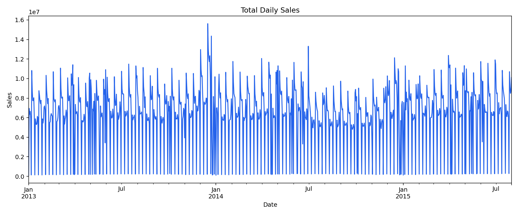
Total Daily Sales
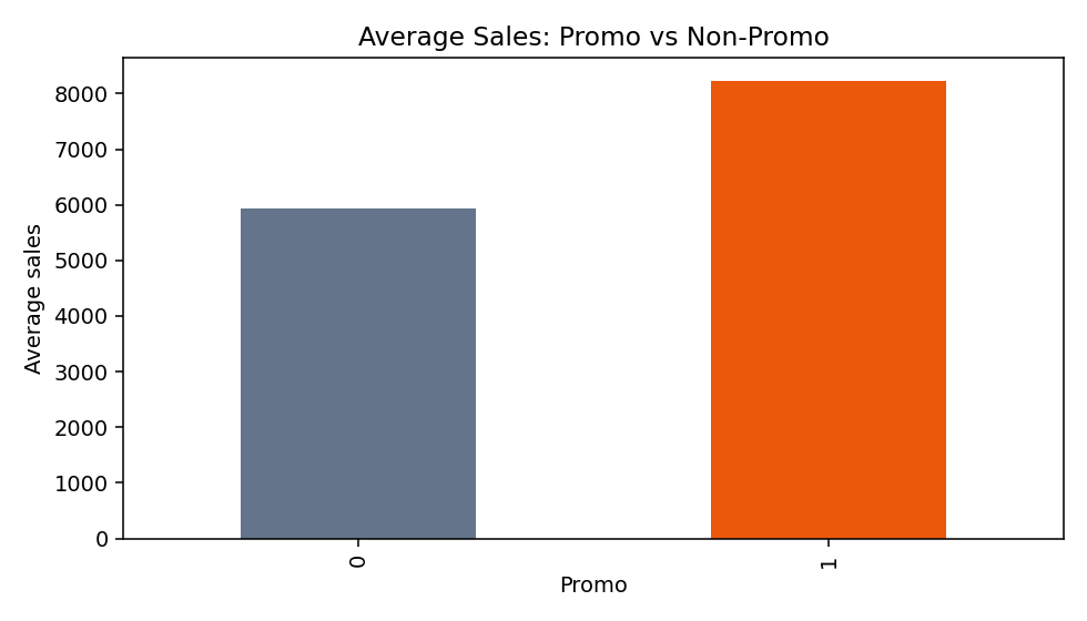
Promotion Lift
Dashboard
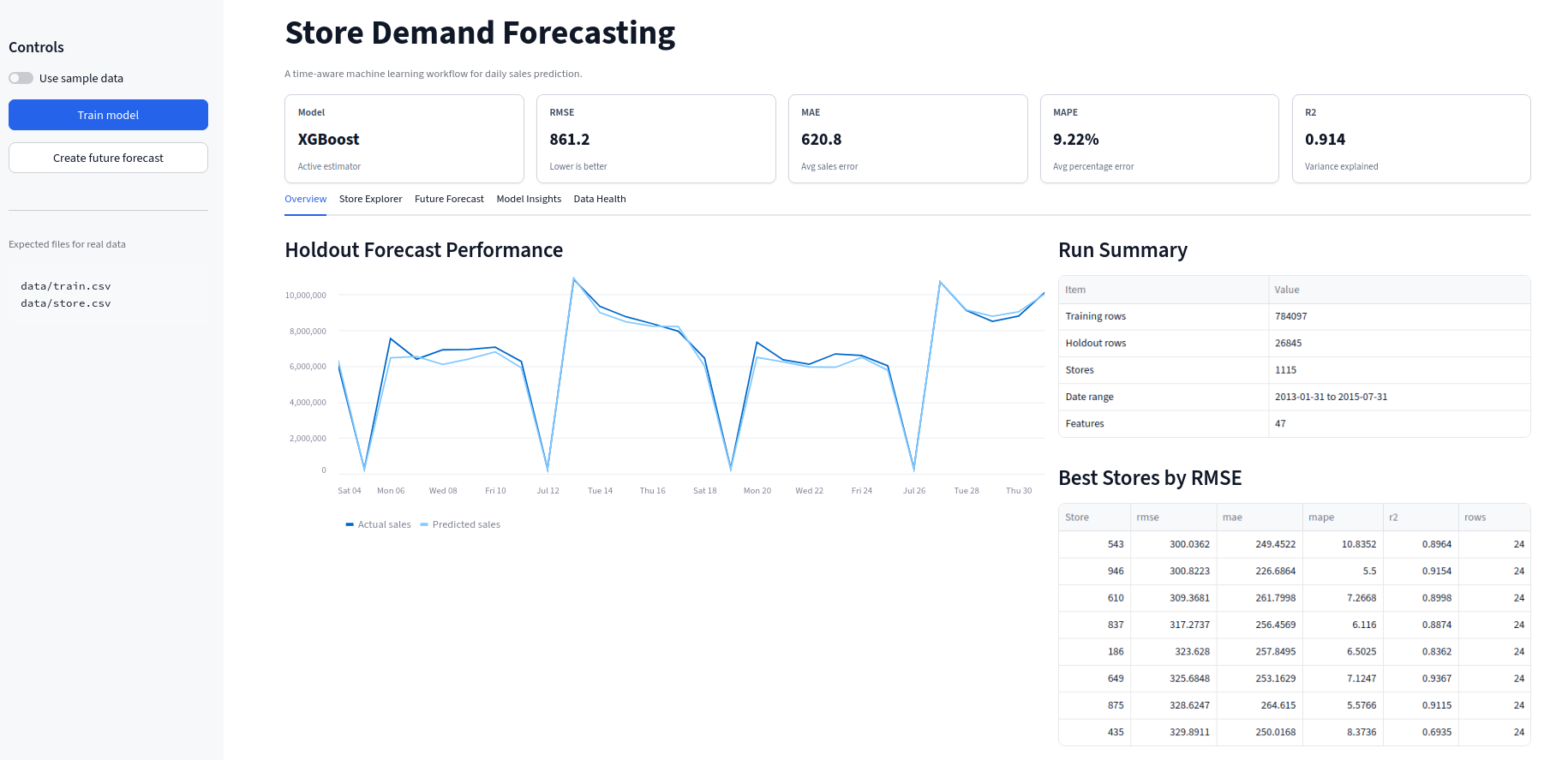
The Streamlit dashboard includes:
- Overview
- Store Explorer
- Future Forecast
- Model Insights
- Data Health
Run it locally:
make dashboard
Repository Structure
demand-forecasting/
├── .streamlit/config.toml
├── app/
│   └── dashboard.py
├── config/
│   └── config.yaml
├── data/
│   └── sample/
├── docs/
│   ├── assets/plots/
│   ├── DATA_GUIDE.md
│   ├── DEPLOYMENT.md
│   ├── EDA_REPORT.md
│   └── RESULTS.md
├── src/
├── tests/
├── Dockerfile
├── docker-compose.yml
├── Makefile
├── TECHNICAL_NOTES.md
└── requirements.txt
Quick Start With Sample Data
python -m venv .venv
source .venv/bin/activate
pip install -r requirements.txt
make train-sample
make eda-sample
make test
make dashboard
Real Data Workflow
Download the Rossmann Store Sales dataset from Kaggle and place:
data/train.csv
data/store.csv
data/test.csv
Then run:
make train
make forecast
make eda
make evaluate
make dashboard
Main Outputs
Generated locally:
models/demand_model.joblib
models/metrics.json
models/holdout_predictions.csv
models/store_metrics.csv
models/feature_importance.csv
models/future_forecast.csv
models/kaggle_submission.csv
models/baseline_comparison.csv
Public report outputs:
docs/EDA_REPORT.md
docs/assets/plots/daily_sales.png
docs/assets/plots/sales_by_weekday.png
docs/assets/plots/promo_lift.png
docs/assets/plots/top_stores.png
Model artifacts and real data stay local. Public docs and plots are safe to push.
Commands
make sample          # generate sample data
make eda             # generate EDA report and plots
make eda-sample      # generate sample-data EDA report and plots
make train-sample    # train with sample data
make train           # train with real data
make forecast        # forecast rows in data/test.csv
make forecast-sample # create sample future forecast
make evaluate        # print saved metrics
make test            # run unit tests
make dashboard       # launch Streamlit
make docker-build    # build local Docker image
make docker-run      # run dashboard from Docker
make clean           # remove generated artifacts
Docker
make docker-build
make docker-run
Or:
docker compose up --build
Next Steps
Good future improvements:
- hyperparameter tuning with Optuna
- SHAP explanations
- MLflow experiment tracking
- FastAPI prediction endpoint
- scheduled retraining
- drift monitoring
Documentation
- docs/DATA_GUIDE.md: data download and setup
- docs/EDA_REPORT.md: exploratory analysis and plots
- docs/RESULTS.md: metrics and interpretation
- docs/DEPLOYMENT.md: Docker and Streamlit deployment
- TECHNICAL_NOTES.md: implementation details